异常检测教程:使用Python进行异常检测的完整指南
技术背景
在日志监控、内容审核、金融风控等场景中,异常检测用于从海量数据中识别偏离正常模式的样本。传统方法依赖手工特征或统计规则,难以捕捉文本语义层面的异常。嵌入模型将文本映射为高维向量,使语义相近的样本在向量空间中聚集,从而可以用距离度量发现离群点。Gemini API 提供多种任务类型的嵌入,适合聚类与异常检测。该方案适用于无标签或弱标签场景,但受限于嵌入模型选择、阈值敏感性和高维距离度量退化等问题。
核心原理
核心流程为:文本经嵌入模型编码为 3072 维向量,使用 CLUSTERING 任务类型使向量适配聚类;随后用 t-SNE 将高维向量降至二维以便可视化,同时保留局部邻域结构;对每个类别计算嵌入质心,再计算样本到所属类别质心的欧氏距离,超过设定半径即判定为异常。数据流为:原始文本→清洗→采样→嵌入→降维→质心→距离→阈值→异常标记。关键设计决策包括固定嵌入模型以保证向量兼容、按类别分别计算质心以处理多簇分布、以及通过距离-异常数量曲线选择阈值。
架构分析
系统由数据层、嵌入层、分析层和可视化层组成。数据层负责加载 20 Newsgroups 并清洗文本;嵌入层封装 Gemini API 调用,通过 progress_apply 批量生成向量并缓存到 DataFrame;分析层实现质心计算与欧氏距离检测,支持参数化半径;可视化层用 t-SNE 投影并用散点图叠加质心与异常点。组件间通过 Pandas DataFrame 传递数据,嵌入向量以 list[float] 存储,便于复用与调试。设计上强调模型固定、任务类型明确、阈值可调,便于在生产中替换为流式处理或向量数据库。
完整实战教程
##### 版权所有 2026 Google LLC。
# @title Licensed under the Apache License, Version 2.0 (the "License");
#
# Licensed under the Apache License, Version 2.0 (the "License");
# you may not use this file except in compliance with the License.
# You may obtain a copy of the License at
#
#     https://www.apache.org/licenses/LICENSE-2.0
#
# Unless required by applicable law or agreed to in writing, software
# distributed under the License is distributed on an "AS IS" BASIS,
# WITHOUT WARRANTIES OR CONDITIONS OF ANY KIND, either express or implied.
# See the License for the specific language governing permissions and
# limitations under the License.
使用嵌入进行异常检测
<a target="_blank" href="https://colab.research.google.com/github/google-gemini/cookbook/blob/main/examples/anomaly_detection.ipynb">
 </a>
</a>
注意: 本笔记本需要付费层级的速率限制才能正常运行。(更多详情请参阅定价)。
概述
本教程演示如何使用 Gemini API 的嵌入来检测数据集中潜在的异常值。你将使用 t-SNE{:.external} 对 20 Newsgroup 数据集的一个子集进行可视化,并检测每个类别簇中心点特定半径之外的异常值。
有关如何开始使用 Gemini API 生成的嵌入的更多信息,请查看快速入门。
前提条件
你可以在 Google Colab 中运行此快速入门。
要在你自己的开发环境中完成此快速入门,请确保你的环境满足以下要求:
- Python 3.11+
- 已安装
jupyter以运行笔记本。
设置
首先,下载并安装 Gemini API Python 库。
%pip install -U -q google-genai seaborn scikit-learn pandas matplotlib
import re
import tqdm
import numpy as np
import pandas as pd
import matplotlib.pyplot as plt
import seaborn as sns

from google import genai
from google.genai import types

# Used to securely store your API key
from google.colab import userdata

from sklearn.datasets import fetch_20newsgroups
from sklearn.manifold import TSNE
获取 API 密钥
在使用 Gemini API 之前,你必须先获取一个 API 密钥。如果你还没有,可以在 Google AI Studio 中一键创建密钥。
<a class="button button-primary" href="https://aistudio.google.com/app/apikey" target="_blank" rel="noopener noreferrer">获取 API 密钥</a>
在 Colab 中,将密钥添加到左侧面板“🔑”下的密钥管理器中。将其命名为 GEMINI_API_KEY。
获取 API 密钥后,将其传递给 SDK。你可以通过两种方式完成:
* 将密钥放入 GEMINI_API_KEY 环境变量中(SDK 会自动从那里读取)。
* 将密钥传递给 genai.Client(api_key=...)
# Or use `os.getenv('GEMINI_API_KEY')` to fetch an environment variable.
GEMINI_API_KEY=userdata.get('GEMINI_API_KEY')

client = genai.Client(api_key=GEMINI_API_KEY)
关键点:接下来,你需要选择一个模型。任何嵌入模型都适用于本教程,但在实际应用中,重要的是选择一个特定的模型并坚持使用。不同模型的输出彼此不兼容。
for m in client.models.list():
  if 'embedContent' in m.supported_actions:
    print(m.name)
选择要使用的模型
MODEL_ID = "gemini-embedding-001" # @param ["gemini-embedding-2-preview", "gemini-embedding-001"] {"allow-input":true, isTemplate: true}
准备数据集
20 Newsgroups 文本数据集{:.external} 包含 18,000 篇关于 20 个主题的新闻组帖子,分为训练集和测试集。训练集和测试集之间的划分基于在特定日期之前和之后发布的消息。本教程使用训练子集。
newsgroups_train = fetch_20newsgroups(subset='train')

# View list of class names for dataset
newsgroups_train.target_names
这是训练集中的第一个示例。
idx = newsgroups_train.data[0].index('Lines')
print(newsgroups_train.data[0][idx:])
# Apply functions to remove names, emails, and extraneous words from data points in newsgroups.data
newsgroups_train.data = [re.sub(r'[\w\.-]+@[\w\.-]+', '', d) for d in newsgroups_train.data] # Remove email
newsgroups_train.data = [re.sub(r"\([^()]*\)", "", d) for d in newsgroups_train.data] # Remove names
newsgroups_train.data = [d.replace("From: ", "") for d in newsgroups_train.data] # Remove "From: "
newsgroups_train.data = [d.replace("\nSubject: ", "") for d in newsgroups_train.data] # Remove "\nSubject: "

# Cut off each text entry after 5,000 characters
newsgroups_train.data = [d[0:5000] if len(d) > 5000 else d for d in newsgroups_train.data]
# Put training points into a dataframe
df_train = pd.DataFrame(newsgroups_train.data, columns=['Text'])
df_train['Label'] = newsgroups_train.target
# Match label to target name index
df_train['Class Name'] = df_train['Label'].map(newsgroups_train.target_names.__getitem__)

df_train
接下来,从训练数据集中抽取 150 个数据点并选择几个类别来对数据进行采样。本教程使用科学类别。
# Take a sample of each label category from df_train
SAMPLE_SIZE = 150
df_train = (df_train.groupby('Label', as_index = False)
                    .apply(lambda x: x.sample(SAMPLE_SIZE))
                    .reset_index(drop=True))

# Choose categories about science
df_train = df_train[df_train['Class Name'].str.contains('sci')]

# Reset the index
df_train = df_train.reset_index()
df_train
df_train['Class Name'].value_counts()
生成嵌入
在本节中,你将了解如何使用 Gemini API 的嵌入模型为数据框中的不同文本生成嵌入。
Gemini 嵌入模型支持多种任务类型,每种类型都针对特定目标而设计。以下是可用类型及其应用场景的总体概览:
任务类型 | 描述
- -- | ---
RETRIEVAL_QUERY | 指定给定文本是搜索/检索场景中的查询。
RETRIEVAL_DOCUMENT | 指定给定文本是搜索/检索场景中的文档。
SEMANTIC_SIMILARITY | 指定给定文本将用于语义文本相似度(STS)。
CLASSIFICATION | 指定嵌入将用于分类。
CLUSTERING | 指定嵌入将用于聚类。
from tqdm.auto import tqdm
tqdm.pandas()

def make_embed_text_fn(model):

  def embed_fn(text: str) -> list[float]:
    # Set the task_type to CLUSTERING.
    result = client.models.embed_content(model=model,
                                            contents=text,
                                            config=types.EmbedContentConfig(
                                                task_type="CLUSTERING"))
    return np.array(result.embeddings[0].values)

  return embed_fn

def create_embeddings(df):
  df['Embeddings'] = df['Text'].progress_apply(make_embed_text_fn(MODEL_ID))
  return df

df_train = create_embeddings(df_train)
df_train.drop('index', axis=1, inplace=True)
降维
文档嵌入向量的维度为 3072。为了可视化嵌入文档是如何分组在一起的,你需要应用降维,因为你只能在 2D 或 3D 空间中可视化嵌入。上下文相似的文档在空间中应该比不相似的文档更接近。
len(df_train['Embeddings'][0])
# Convert df_train['Embeddings'] Pandas series to a np.array of float32
X = np.array(df_train['Embeddings'].to_list(), dtype=np.float32)
X.shape
你将应用 t-分布随机邻域嵌入(t-SNE)方法来进行降维。该技术减少了维度数量,同时保留了聚类(彼此靠近的点仍然保持靠近)。对于原始数据,模型尝试构建一个关于哪些其他数据点是“邻居”的分布(例如,它们具有相似的含义)。然后,它优化一个目标函数,以在可视化中保持相似的分布。
tsne = TSNE(random_state=0)
tsne_results = tsne.fit_transform(X)
df_tsne = pd.DataFrame(tsne_results, columns=['TSNE1', 'TSNE2'])
df_tsne['Class Name'] = df_train['Class Name'] # Add labels column from df_train to df_tsne
df_tsne
fig, ax = plt.subplots(figsize=(8,6)) # Set figsize
sns.set_style('darkgrid', {"grid.color": ".6", "grid.linestyle": ":"})
sns.scatterplot(data=df_tsne, x='TSNE1', y='TSNE2', hue='Class Name', palette='Set2')
sns.move_legend(ax, "upper left", bbox_to_anchor=(1, 1))
plt.title('Scatter plot of news using t-SNE')
plt.xlabel('TSNE1')
plt.ylabel('TSNE2')
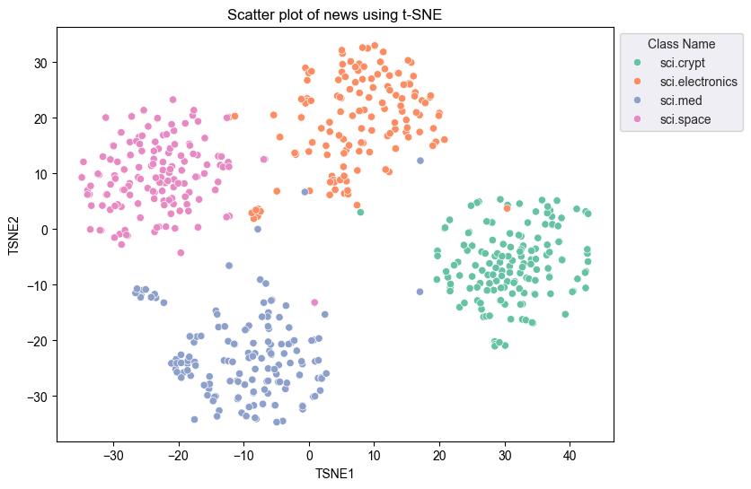
异常检测
要确定哪些点是异常的,你需要确定哪些点是内点,哪些是外点。首先找到质心,即代表聚类中心的位置,然后利用距离来确定哪些点是外点。
首先获取每个类别的质心。
def get_centroids(df_tsne):
  # Get the centroid of each cluster
  centroids = df_tsne.groupby('Class Name').mean()
  return centroids

centroids = get_centroids(df_tsne)
centroids
def get_embedding_centroids(df):
  emb_centroids = dict()
  grouped = df.groupby('Class Name')
  for c in grouped.groups:
    sub_df = grouped.get_group(c)
    # Get the centroid value of dimension 768
    emb_centroids[c] = np.mean(sub_df['Embeddings'], axis=0)

  return emb_centroids
emb_c = get_embedding_centroids(df_train)
将你找到的每个质心与其余点绘制在一起。
# Plot the centroids against the cluster
fig, ax = plt.subplots(figsize=(8,6)) # Set figsize
sns.set_style('darkgrid', {"grid.color": ".6", "grid.linestyle": ":"})
sns.scatterplot(data=df_tsne, x='TSNE1', y='TSNE2', hue='Class Name', palette='Set2');
sns.scatterplot(data=centroids, x='TSNE1', y='TSNE2', color="black", marker='X', s=100, label='Centroids')
sns.move_legend(ax, "upper left", bbox_to_anchor=(1, 1))
plt.title('Scatter plot of news using t-SNE with centroids')
plt.xlabel('TSNE1')
plt.ylabel('TSNE2');
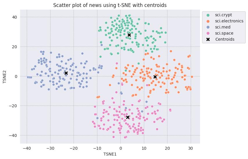
选择一个半径。任何超出该类别质心此范围的样本都被视为异常值。
def calculate_euclidean_distance(p1, p2):
  return np.sqrt(np.sum(np.square(p1 - p2)))

def detect_outlier(df, emb_centroids, radius):
  for idx, row in df.iterrows():
    class_name = row['Class Name'] # Get class name of row
    # Compare centroid distances
    dist = calculate_euclidean_distance(row['Embeddings'],
                                        emb_centroids[class_name])
    df.at[idx, 'Outlier'] = dist > radius

  return len(df[df['Outlier'] == True])
range_ = np.arange(0.3, 0.75, 0.02).round(decimals=2).tolist()
num_outliers = []
for i in range_:
  num_outliers.append(detect_outlier(df_train, emb_c, i))
# Plot range_ and num_outliers
fig = plt.figure(figsize = (14, 8))
plt.rcParams.update({'font.size': 12})
plt.bar(list(map(str, range_)), num_outliers)
plt.title("Number of outliers vs. distance of points from centroid")
plt.xlabel("Distance")
plt.ylabel("Number of outliers")
for i in range(len(range_)):
  plt.text(i, num_outliers[i], num_outliers[i], ha = 'center')

plt.show()
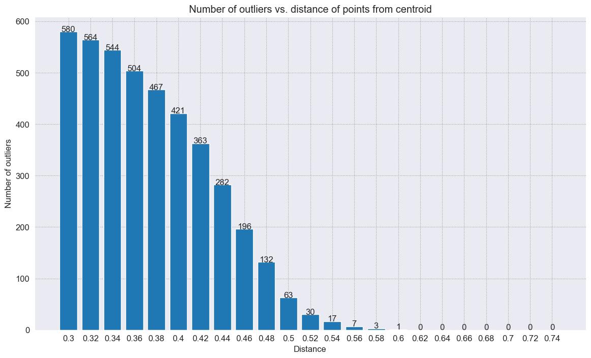
根据你希望异常检测器的敏感程度,你可以选择要使用的半径。目前使用的是 0.58,但你可以更改这个值。
# View the points that are outliers
RADIUS = 0.54
detect_outlier(df_train, emb_c, RADIUS)
df_outliers = df_train[df_train['Outlier'] == True]
df_outliers.head()
# Use the index to map the outlier points back to the projected TSNE points
outliers_projected = df_tsne.loc[df_outliers['Outlier'].index]
绘制离群点,并使用透明红色标记它们。
fig, ax = plt.subplots(figsize=(8,6)) # Set figsize
plt.rcParams.update({'font.size': 10})
sns.set_style('darkgrid', {"grid.color": ".6", "grid.linestyle": ":"})
sns.scatterplot(data=df_tsne, x='TSNE1', y='TSNE2', hue='Class Name', palette='Set2');
sns.scatterplot(data=centroids, x='TSNE1', y='TSNE2', color="black", marker='X', s=100, label='Centroids')
# Draw a red circle around the outliers
sns.scatterplot(data=outliers_projected, x='TSNE1', y='TSNE2', color='red', marker='o', alpha=0.5, s=90, label='Outliers')
sns.move_legend(ax, "upper left", bbox_to_anchor=(1, 1))
plt.title('Scatter plot of news with outliers projected with t-SNE')
plt.xlabel('TSNE1')
plt.ylabel('TSNE2')
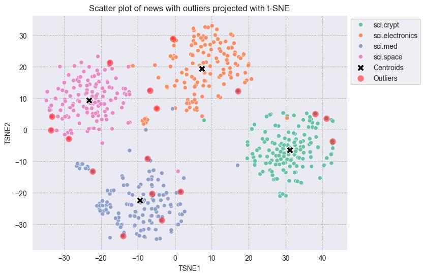
使用数据帧的索引值来打印一些示例,以展示每个类别中异常值可能的样子。这里,打印出每个类别的第一个数据点。探索每个类别中的其他点,以查看被视为异常值或异常的数据。
sci_electronics_outliers = df_outliers[df_outliers['Class Name'] == 'sci.electronics']
print(sci_electronics_outliers['Text'].iloc[0])
sci_space_outliers = df_outliers[df_outliers['Class Name'] == 'sci.space']
print(sci_space_outliers['Text'].iloc[0])
后续步骤
你现在已经使用嵌入创建了一个异常检测器!尝试使用你自己的文本数据,将它们可视化为嵌入,并选择一些边界,以便你可以检测离群值。你可以执行降维以完成可视化步骤。请注意,t-SNE 擅长对输入进行聚类,但可能需要较长时间才能收敛,或者可能会陷入局部最小值。
要了解如何使用 Gemini API 中的其他服务,请参阅入门指南。
常见问题
常见错误包括:API 密钥未设置导致认证失败,需检查 GEMINI_API_KEY 环境变量或 userdata;嵌入模型混用导致向量不兼容,应固定 MODEL_ID;t-SNE 收敛慢或陷入局部最优,可调整 perplexity 或改用 UMAP;阈值选择不当导致异常过多或过少,应结合业务目标与距离分布曲线;高维距离度量失效,可先归一化或使用余弦距离。排查时先验证单条文本嵌入维度,再检查质心计算是否按类别分组,最后可视化距离分布。生产环境建议缓存嵌入、批量请求、设置重试与限流,并考虑用近似最近邻替代全量距离计算。
企业应用扩展
可扩展方向包括:将阈值选择自动化,如基于距离分位数或孤立森林;用向量数据库存储嵌入并支持增量检测;结合多模态嵌入检测图像或音频异常;引入半监督方法利用少量标签提升精度;将 t-SNE 替换为 UMAP 以提升大规模数据性能;在生产中接入监控告警,对异常样本进行人工复核与反馈闭环。
总结
本教程面向有编程基础的开发者,讲解如何利用 Gemini API 的文本嵌入与 t-SNE 降维,在 20 Newsgroups 数据集上构建异常检测器。内容涵盖嵌入生成、任务类型选择、质心计算、欧氏距离阈值判定与可视化,并给出环境准备、代码分析、常见错误排查及生产优化建议,帮助读者掌握基于嵌入的异常检测工程实践。
- --
内容来源与验证
- 内容等级:PREMIUM_A
- 质量等级:A
- 难度:中级
- 验证等级:V1
- 原文作者:
- 原文日期:
- 来源许可:Apache-2.0
- 来源版本:
f76a507a0c1cac0557e732d9865a5b7499922516 - 查看原文
站内还有更多完整实战教程
加入会员,解锁全部教程、完整代码与持续更新内容。
加入会员